
Spectroscopic Microplastics Analysis:
A Complete Overview
Getting Started with Microplastics Analysis
Microplastics analysis has moved fast. What began as a niche topic in marine biology is now a central concern in environmental monitoring, food safety, drinking water regulation, and human health research. Regulatory frameworks are being established. International standards have been published. Laboratories that once approached microplastics as an occasional special project are now building dedicated workflows to handle routine sample volumes.
Which brings us to the fundamental question:
Which analytical approach is the right one for my laboratory?
This guide explains how to choose spectroscopic methods, filter substrates, and data evaluation workflows for particle-based microplastics analysis, with emphasis on practical trade-offs, regulatory relevance, and known analytical limitations.
For a shorter version, start with the FAQ.
Our FAQ distills the most important answers on methods, instrumentation, sample preparation, data evaluation, and the standards shaping the field.
#1 Defining the Microplastics Problem
Microplastics are solid polymer particles smaller than 5 mm, spanning an enormous range from millimeter-scale fragments visible to the naked eye down to particles of 5 to 10 micrometers that require microscopic methods to detect at all.
Within that range, size, shape, and polymer type all carry scientific meaning. The question an analysis must answer is not simply whether microplastics are present, but how many, how large, what shape, and what they are made of.
Microplastics have been detected in ocean surface water and deep-sea sediments, in Arctic ice, in agricultural soil, in indoor air, and in the human food chain. Published studies frequently report the presence of microplastics in tap and bottled water, with observed prevalence varying widely depending on analytical method, particle size threshold, and identification criteria.
In several widely cited surveys, microplastics were reported in up to 87% of analyzed tap water samples globally[1] and in up to 93% of tested bottled water brands.[2] They have also been identified in human lung tissue[3], blood[4], and placenta[5]. Of course, reported detection rates should be interpreted in the context of the analytical approaches and detection limits applied in each study.
In short, the scale of environmental distribution is no longer in question. It is massive.
Primary microplastics are manufactured intentionally (e.g. : cosmetic microbeads, plastic pellets, abrasive blast media) and represent a smaller fraction of the total environmental burden.
Secondary microplastics form through the physical, chemical, and biological degradation of larger plastic objects and account for the vast majority of what environmental samples contain.
Here, tire and road wear particles (TRWP) are widely recognised as one of the largest sources of microplastics released into the environment. Tire and road wear particles are among the major sources of microplastic emissions, and in Germany tire abrasion has been estimated at around 60,000–100,000 t/a, with peer-reviewed modelling studies reporting comparable values of 75,200–98,400 t/a for coarse non-airborne tire wear particles.[7] Other relevant secondary microplastic sources include emissions from waste disposal and plastic packaging, abrasion of asphalt-bound polymers, pellet losses, textile washing, paints, and agricultural plastics.[7]
Nanoplastics, typicall particles below 1 µm, are an emerging focus in toxicology and health research. Their small size allows them to cross biological barriers, including cell membranes and, potentially, the blood-brain barrier.[8] They are challenging samples and usually require a more time-consuming analytical approach than standard microplastics work.
The core analytical challenge across all of these size ranges is the same: environmental samples are complex mixtures. Synthetic polymer particles arrive alongside natural particles, including cellulose fibers, mineral fragments, and biological material. Visual inspection alone cannot distinguish a polyethylene fragment from a cellulose fiber. Chemical identification of each individual particle is not optional. It is the basis of any result that means anything.
What are Microplastics?
| Contaminant Classification | Physical Size Boundaries | Primary Environmental Genesis | Predominant Analytical Challenges | Key Representative Examples |
| Primary Microplastics | 5 µm to 5 mm | Intentionally manufactured for specific industrial functions or consumer product formulations. | Locally concentrated near industrial sites; requires differentiation from secondary background fragments. | Cosmetic microbeads, raw manufacturing resin pellets (nurdles), abrasive blast media. |
| Secondary Microplastics | 5 µm to 5 mm | Progressive physical, chemical, and biological degradation of larger macro-plastic waste. | Extreme structural heterogeneity; often heavily weathered, bio-fouled, or embedded in matrix residues. | Tire and Road Wear Particles (TRWP), synthetic textile wash fibers, fragmented agricultural films. |
| Nanoplastics | Sub-micron (< 1 µm / < 1000 nm) | Advanced fragmentation and continuous degradation of microplastic particles. | Sits below the optical diffraction limit of standard mid-infrared micro-spectroscopy. | Sub-micron polymer colloids, weathered synthetic dusts capable of cellular translocation. |
| Natural/Inorganic Background Matrix | Highly variable (< 0.1 µm to > 5 mm) | Naturally occurring biotic and abiotic environmental components. | Inflicts heavy spectral interference; can completely mimic plastic particles under visual inspection. | Cellulose (cotton/wood fibers), chitin, mineral shards (silica/quartz), bio-films. |
#2 Mass-Driven or Particle-Driven Microplastics Analysis?
Microplastics analysis covers a range of analytical questions, including particle number and size distribution, polymer mass concentration, and chemical composition. No single method can address all of these questions simultaneously. The two dominant approaches in microplastics research are built on different principles and produce fundamentally different outputs.
Mass vs. Particle Metrics
| Metric Category | Primary Technique | Data Output | Core Advantages | Critical Limitations |
| Mass-Driven | Pyrolysis GC/MS (Pyro-GC/MS); TED-GC/MS | Total polymer mass concentration profile (mg/kg or µg/L). | Quantifies total polymer burden; high matrix tolerance. | Destructive; entirely blind to particle count, size distribution, and morphology. Pre-separation via sifting introduces particle loss uncertainties. |
| Particle-Driven | FT-IR Microscopy, Quantum Cascade Laser (QCL) IR, Raman Microscopy | Spatially resolved particle counts, discrete sizing, morphology metrics, and chemical typing. | Matches toxicological exposure models; non-destructive nature permits archival storage and retrospective audit. | Requires rigorous sample preparation to mitigate spectral interference from co-extracted matrices. |
Mass-Driven Analysis
Pyrolysis GC/MS (Pyro‑GC/MS) is an inherently destructive analytical technique. The sample is thermally decomposed, the resulting fragments are separated by gas chromatography, and polymers are identified and quantified by mass spectrometry. The output is a quantitative polymer profile, reporting which polymers are present and their concentrations by mass.[6]
For questions of total polymer burden, Pyro‑GC/MS is therefore a powerful tool. Its fundamental limitation[6] is its indifference to particle size. Simply put: A single large plastic fragment will give the same result as a whole population of particles in various sizes that add up to equal mass.
Once a sample has been pyrolyzed, no particle remains. Size distribution, morphology, fiber versus fragment classification, and particle counts do not survive the analysis, and the sample cannot be archived or reanalyzed.
As a result, for regulatory and biological questions that increasingly drive monitoring efforts, mass‑based methods cannot deliver particle‑level metrics, but they remain valuable for providing complementary polymer mass information.
As a "workaround" to reintroduce some size resolution into mass‑based analyses, size fractionation can be applied prior to chemical measurement. Size fractionation is typically achieved using sieving, filtration cascades, or sequential separation steps, often combined with density separation, to divide samples into discrete size classes before analysis by Pyro‑GC/MS or related techniques (e.g., TED‑GC/MS).
Commonly reported fractions include coarse (>500 or >300 µm), intermediate (100–500 µm), and fine (<100 µm) classes, though exact cutoffs vary depending on matrix, analytical sensitivity, and study objectives.
While this approach does not preserve individual particle identity, it enables attribution of polymer mass to size ranges that are more directly relevant for exposure modeling, transport behavior, and risk‑oriented assessments.
However, size fractionation itself introduces additional sources of uncertainty that must be considered. Particle losses can occur during sieving or filtration due to adhesion to equipment surfaces, clogging, or incomplete transfer between steps, with fine and fibrous particles being particularly susceptible.
Mechanical handling may also induce fragmentation or deformation, altering the apparent size distribution. Therefore, size‑fractionated mass‑based methods are infrequently applied in microplastics research, largely due to the field’s emphasis on particle‑level identification.
This guide focuses on particle‑driven microplastics analysis.
We are focusing on the analytical metrics currently applied in regulatory and standardisation frameworks and the type of information generated by particle-driven analysis techniques. In practice, however, particle‑driven and mass‑driven methods are often used in combination, depending on the analytical objectives and regulatory context.
Particle-Driven Analysis
Infrared (IR) and Raman microscopy are inherently particle‑resolved techniques. The sample remains intact, with particles immobilized on a filter and analyzed individually or as a complete population. The analytical output is particle‑level information, including polymer identity, size, morphology, and particle count for each detected item on the filter. This matters for two reasons:
- It reflects how microplastics interact with biological systems. Particle size, shape, and form directly influence transport, deposition, and biological response: a 10 µm fiber and a 500 µm fragment of the same polymer represent fundamentally different exposure scenarios. Likewise, a high abundance of small particles conveys different biological and toxicological implications than a low abundance of larger particles. Collapsing these distinctions into a single mass‑based metric obscures the parameters that drive exposure assessment and risk evaluation.
- The non‑destructive nature of spectroscopic analysis allows samples to be archived. Filters analyzed today remain available for reanalysis under future regulatory requirements, revised size classifications, or updated polymer libraries, without the need to recollect the original sample. As regulatory and standardisation frameworks continue to evolve, this capacity for retrospective analysis represents a significant operational and scientific advantage.
Accordingly, regulatory frameworks have increasingly adopted particle‑based metrics that require information on particle number, size distribution, and morphology. EU Commission Delegated Decision (EU) 2024/1441, implementing the Drinking Water Directive (EU) 2020/2184, specifies a harmonised methodology for microplastics measurement in drinking water based on particle‑level characterisation using vibrational micro‑spectroscopy.
ISO 24187:2023 adopts a similar perspective by defining general principles for particle‑based microplastics analysis across environmental matrices, including water, sediment, and biota. In these frameworks, microplastics are reported primarily in terms of particle counts and size classes rather than total polymer mass.
Particle‑driven analysis therefore depends on the capability of a technique to provide chemical identification of individual particles without destroying them, an intrinsic value of vibrational micro spectroscopy. Here, each polymer exhibits a characteristic spectral fingerprint, enabling discrimination of plastic and non-plastic, synthetic and natural, and even between the polymer types of particles.
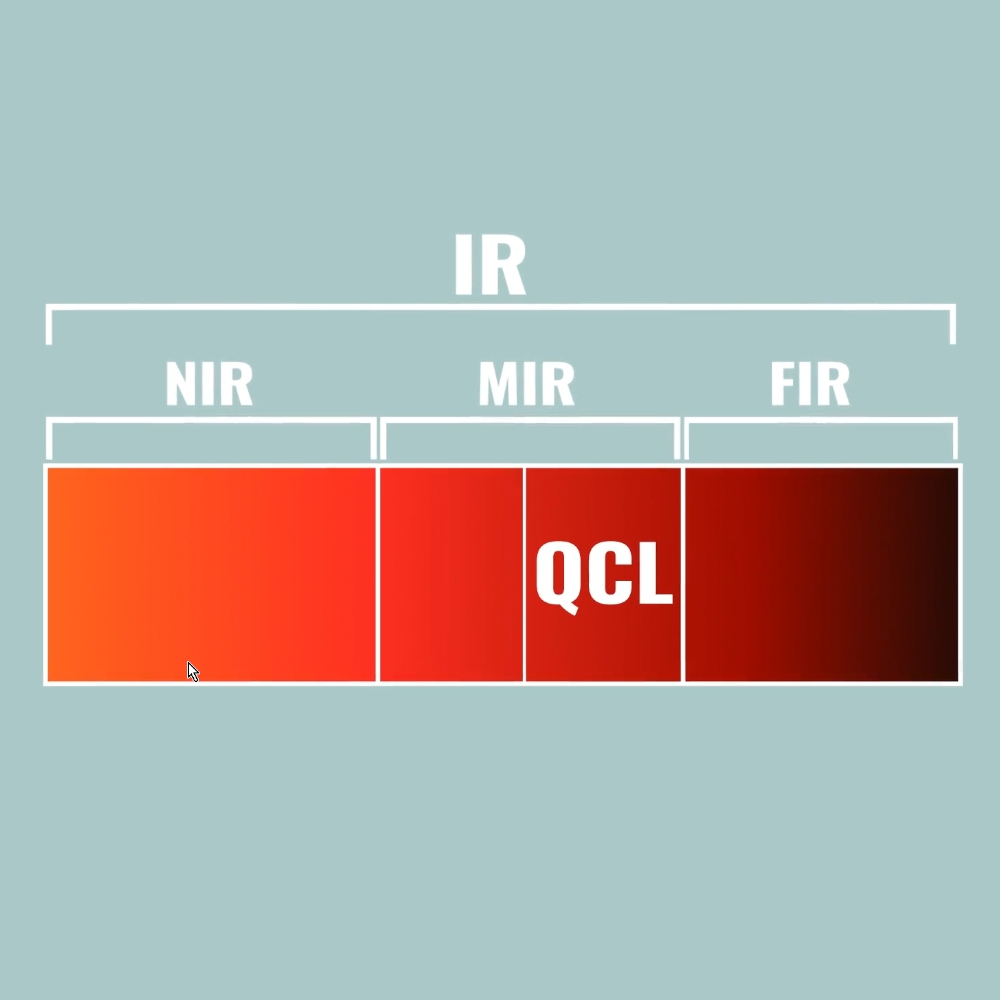
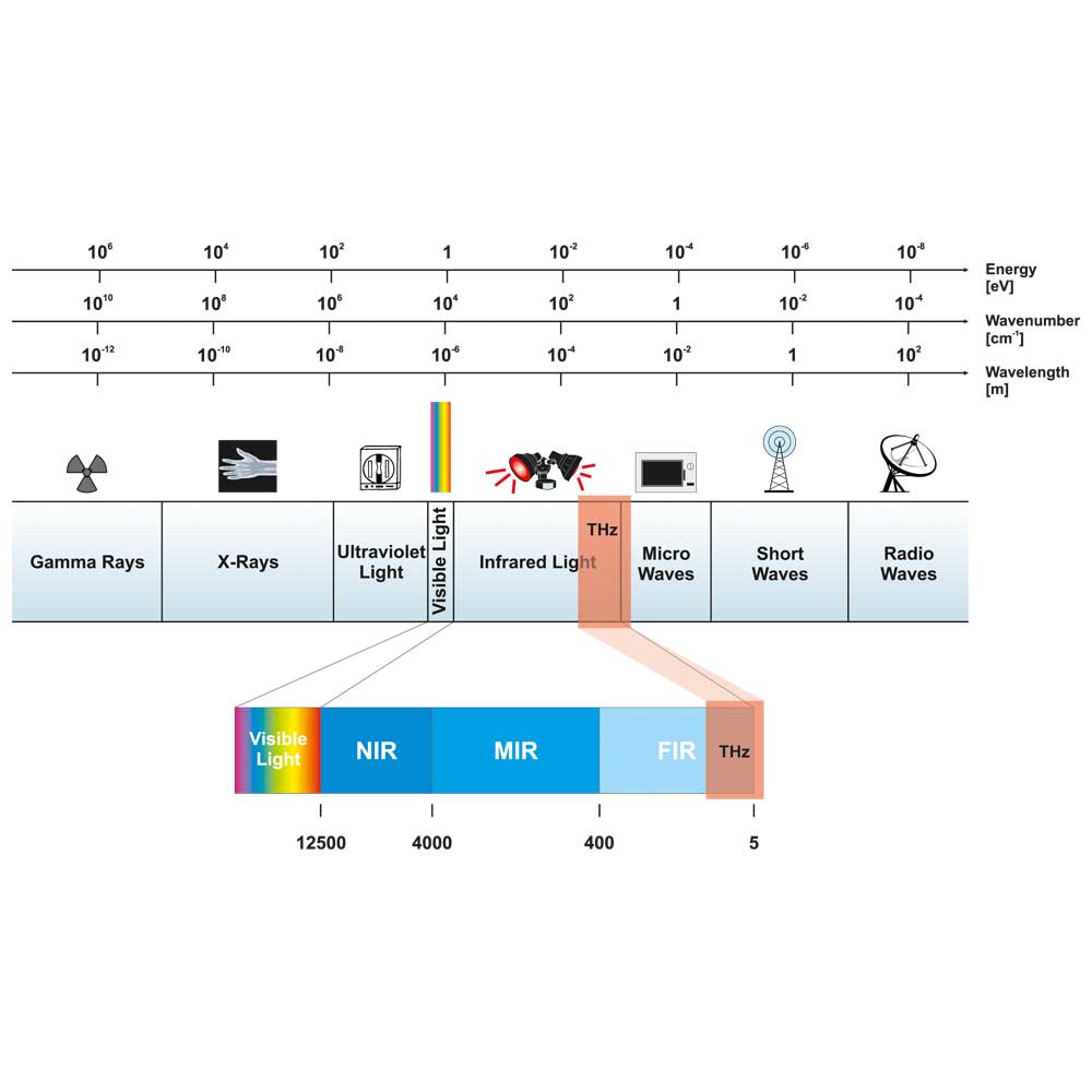
FT-IR, IR laser, and Raman microscopy all identify particles through vibrational spectra, but they differ in spatial resolution, throughput, spectral coverage, and minimum reliable particle size. The choice between these techniques is therefore not arbitrary and is addressed in detail in the technique‑specific sections.
All three follow the same workflow: sample collection, preparation, filtration, spectroscopic measurement, and data evaluation. The major analytical distinction is whether spectra are acquired from optically selected particles one by one, or from a spatially resolved chemical image of a defined filter area.
#3 The Analytical Workflow
Spectroscopic microplastics analysis follows the same five-step sequence regardless of which technique is used and each step, to some degree, will affect data quality.
Step 1: Sample Collection
Representative sampling is the foundation of any valid result. Errors introduced here cannot be corrected downstream by even the most precise spectroscopic analysis. What constitutes representative sampling varies considerably by matrix: surface water, sediment, biological tissue, drinking water, and food products each require their own approach. Contamination prevention is essential at this stage, from equipment choice through to procedural blanks and working environment.
However, exact sampling protocols are outside the scope of this guide.
For general principles of microplastics analysis, see ISO 24187:2023. For drinking water and waters with low suspended-solids content, see ISO 16094-2:2025.

Step 2: Sample Preparation
Sample preparation is arguably the most critical step in the entire workflow and the primary source of variability between laboratories. Its complexity depends entirely on the matrix. Drinking water may require little more than direct filtration. Ocean sediment, biological tissue, or food products each require their own approach to remove organic and inorganic matrix material that would otherwise interfere with spectroscopic analysis or produce false identifications.
Common techniques include density separation to remove mineral particles, chemical digestion to destroy organic matter, and sequential sieving for size fractionation. The goal is a clean suspension of particles ready for filtration, with matrix material maximally removed without damaging the plastic particles themselves.
Neither measurement nor software can compensate for inadequate preparation. What arrives on the filter is what the instrument sees, and the old adage still applies: "Garbage in, garbage out."
This guide does not cover sample preparation protocols in detail. For method-specific guidance, see ISO 24187:2023 which addresses preparation requirements for environmental samples.

Step 3: Filtration and Filter Selection
The prepared suspension is filtered onto a substrate, and the choice of that substrate is closely linked to the analytical technique used. It determines which measurement modes are available, affects spectral quality, and controls whether the smallest particles are captured quantitatively. It is a decision that needs to be made deliberately and early, because changing filter type mid-study is never a wise choice.
Filter selection is covered in full on its dedicated section.

Step 4: Spectroscopic Measurement
The loaded filter is transferred to the instrument and measured. Independent of the technique, the measurement aims at acquiring molecular vibration spectra encoding the chemical identity of every particle on the filter. Each technique operates differently in terms of light source, detection principle, spatial resolution, and throughput, with real consequences for what the data can and cannot tell you.
FT-IR microscopy, IR laser microscopy, and Raman microscopy differ mainly in source, detection principle, resolution, and throughput. Each technique can be used either for selected-particle spectroscopy or for spatially resolved chemical imaging.
This distinction between micro-spectroscopy and spectroscopic imaging becomes central in Section 5.

Step 5: Data Evaluation
The task of data evaluation is to turn the collected measurement data into results in terms of particle count, size, and identity. Data evaluation differs considerably depending on the measurement approach, e.g. whether only single spectra are measured or a full chemical image consisting of millions of spectra is acquired.
A common requirement for all scenarios is to infer the identity of a polymer from the measured spectrum. Classical library matching, the traditional approach, often performs poorly on real-world environmental samples. AI models trained on large datasets of real-world microplastic spectra can handle this task substantially better.
The role of data evaluation software, and what to look for in it, is covered in its own section.

| Workflow Phase | Core Analytical Objective | Dominant Reagents & Hardware | Critical Data Quality Hazards | Quality Assurance & Mitigation Controls |
| 1. Sample Collection | Gathering a statistically representative sample while eliminating background contaminants. | Neuston nets, stainless-steel grabs, glass containers, bypass filter rigs. | Airborne synthetic fiber fallout; cross-contamination from plastic sampling gear. | Mandatory execution of field and procedural blank filters; absolute exclusion of consumer plastic clothing/gear. |
| 2. Sample Preparation | Complete isolation of target polymers via mineral separation and organic destruction. | High-density salts (ZnCl2, NaI); oxidative solutions (H2O2, Fenton's reagent); enzymes. | Chemical degradation or melting of vulnerable polymers; particle loss via physical handling errors. | Precise temperature caps (< 40–50°C); use of non-destructive enzymatic cascades or specialized catalyst controls. |
| 3. Filtration | Concentrating isolated particles onto an optically compatible substrate disc. | Glass vacuum filter assemblies; Anodisc, Silicon, or Metal-coated polycarbonate discs. | Particle clustering/clogging; substrate distortion; passage of fine particles through oversized pores. | Careful calculation of split-sample loading densities; optimization of substrate pore size configurations (0.2 µm). |
| 4. Spectroscopic Measurement | Acquiring descriptive molecular vibration signatures from target particles. | FT-IR, IR Laser, and Raman microscopes. | Signal-to-noise degradation; thermal degradation from over-powered lasers; background interference. | Optimization of scan integration parameters; execution of daily background single-beam reference scans. |
| 5. Data Evaluation | Converting raw spectral arrays into verified particle counts and morphology lists. | Automated baseline algorithms; library search engines; trained neural networks. | False positives from weathered profiles; false negatives; sizing errors due to overlapping particles. | Utilization of machine learning models trained on heavily degraded real-world polymers; strict verification thresholds. |
#4 Filter Substrates: Matching the Filter to the Method
In microplastics analysis, a filter does two jobs simultaneously. It captures the particles from your prepared sample, and sits directly in the optical path of the spectroscopic measurement. That second role is what makes substrate selection consequential in a way that goes beyond simple compatibility.
The filter material inevitably interacts with the IR beam or the Raman laser during measurement. IR transmission measurements requires an IR-transparent material. Raman microscopy needs a flat substrate that does not fluoresce under laser excitation.
Its optical properties determine how much of the spectral range is accessible, how strong the signal is, and whether the substrate itself contributes unwanted background to the spectrum.
Pore size determines the smallest particle retained quantitatively. Surface chemistry affects how well particles adhere during handling. Consequences of unguided filter selection range from degraded spectral quality to lost particles to a measurement mode that simply cannot work on the substrate you have chosen. Filter selection is a decision that needs to be made before filtration, based on the analytical technique being used downstream.

Filter Compatibility at a Glance
| Filter | IR Transmission | IR Transflection | ATR | Raman | Pore size |
| Anodisc | Best | No | No | No (fluoresces, rough) | 20 nm |
| Silicon | Yes | Yes | No | Yes | 1-50 µm |
| Metal/Polycarbonate | No | Best | Yes | Best | 0.1 µm |
| PTFE | Partial | No | Yes | Partial | Various |
| Nitrocellulose | No | No | Yes | No (burns) | Various |
| Glass fiber | No | No | Yes | With caution | Various |
Anodisc (Aluminum Oxide Membrane)
Anodisc filters are the de facto standard substrate for infrared transmission‑based microplastics analysis. The aluminum oxide membrane is highly transparent above approximately 1250 cm⁻¹, fully covering the polymer fingerprint region required for routine identification of all major plastic types.
Below this threshold the membrane becomes opaque, which represents a defined but generally acceptable limitation, as polymer classification rarely relies on spectral features in this range. With a standard pore size of 0.2 µm, Anodisc filters retain all particles that can be reliably characterized by IR microscopy. They are cost‑effective and straightforward to handle, although their ceramic structure makes them mechanically brittle.
While being well suited for IR measurements, Anodisc filters are incompatible with Raman spectroscopy. The aluminum oxide matrix exhibits strong laser‑induced fluorescence, which overwhelms Raman signals and renders the substrate unsuitable for Raman‑based particle identification. Additionally, the high roughness complicates the measurements especially at high resolutions for nanoplatics
- Compatible with: IR transmission
- Not suitable for: Raman

Silicon Membrane Filters
Silicon membrane filters provide full mid‑infrared transmission across approximately 4000–600 cm⁻¹, extending well below the lower cutoff of aluminum oxide membranes. This expanded spectral access becomes relevant when inorganic components must be characterized alongside polymers, as materials such as glass exhibit diagnostic absorption features in this region. In contrast to Anodisc, silicon substrates are also fully compatible with Raman spectroscopy and do not introduce fluorescence interference.
This extended functionality comes at the cost of analytical efficiency. Silicon absorbs a portion of the incident IR radiation, necessitating longer acquisition times to achieve signal‑to‑noise ratios comparable to those obtained with aluminum oxide membranes. For routine polymer identification, this additional measurement time is rarely justified. Silicon filters are therefore best reserved for applications where access to the full mid‑infrared range or combined IR–Raman analysis is analytically required.
- Compatible with: IR transmission, Raman
- Best suited for analyses requiring full MIR coverage or identification of inorganic components

Metal-Coated Polycarbonate Filters
Metal‑coated polycarbonate filters (e.g. gold-coated) are purpose‑designed substrates for IR transflection and Raman spectroscopy. They are not suitable for IR transmission measurements. In Raman applications, the metal coating provides an inert, non‑fluorescent surface that produces neither Raman scattering nor background fluorescence, yielding exceptionally clean spectra. Pore sizes down to 0.1 µm are available, ensuring retention of all particles within the spectroscopically accessible size range.
In IR transflection mode, the reflective metal layer creates a double‑pass optical geometry that can enhance signal intensity for small or thin particles. However, for larger particles this can lead to early spectral saturation, limiting quantitative interpretability. Furthermore, as the resulting spectra have components of both, transmission and reflection signals, the spectral quality is generally inferior to pure transmission measurements which may adversely affect identification.
- Compatible with: IR transflection, Raman
- Not suitable for: IR transmission

PTFE Membranes
PTFE membranes transmit infrared radiation adequately above approximately 1300 cm⁻¹ but exhibit a strong absorption band between 1100 and 1300 cm⁻¹ that partially overlaps the polymer fingerprint region. This creates a spectral gap that can interfere with confident polymer identification. PTFE filters are inexpensive and widely available, but their primary limitation is mechanical rather than optical: particles adhere weakly to the hydrophobic surface and can be lost during handling, transfer, or storage.
For applications where quantitative accuracy or particle retention is critical, this detachment risk represents a non‑trivial source of uncertainty.
- Compatible with: IR transmission (with limitations), ATR
- Key limitations: spectral gap in fingerprint region, particle adhesion and loss

Nitrocellulose Filters
Nitrocellulose membranes are widely used in general laboratory filtration but have very limited applicability in microplastics workflows. Strong intrinsic IR absorption renders them incompatible with transmission and transflection imaging, restricting IR measurements to ATR only. They are unsuitable for Raman spectroscopy, as laser exposure can thermally damage or ignite the membrane. As a result, nitrocellulose filters cannot be used in automated, full‑filter imaging workflows.
- Compatible with: ATR
- Not suitable for: IR transmission, IR transflection, Raman, automated imaging

Glass Fiber
Glass fiber filters exhibit IR limitations similar to nitrocellulose membranes: strong absorption prevents transmission and transflection measurements, leaving ATR as the only viable IR option. For Raman spectroscopy they can be used, but with caution, as the glass fibers contribute their own Raman scattering background, which can complicate spectral interpretation and polymer discrimination. Like nitrocellulose, glass fiber filters are unsuitable for automated full‑filter imaging approaches.
- Compatible with: ATR
- Raman: usable with caution; background contribution must be accounted for
- Not suitable for automated imaging workflow
#5 Micro-Spectroscopy and Imaging: A Fundamental Difference for Microplastics
So far, we have referred to FT-IR microscopy, IR laser microscopy, and Raman microscopy as the main spectroscopic techniques for particle-driven microplastics analysis. For microplastics work, it is useful to distinguish between micro-spectroscopy and spectroscopic imaging, because the expectations placed on the resulting data are fundamentally different.
For particle-based microplastics analysis, overall, spectroscopic imaging provides the stronger analytical basis when the objective is to generate particle statistics across a defined filter area. The particle population is derived from the chemical dataset itself rather than by prior (unreliable) visual detection.
It goes beyond confirming optically selected particles and enables chemical-data-based localization, counting, sizing, morphology assessment, and polymer identification. At this point subsampling should also be discussed as it is inherently connected to micro-spectroscopic approaches.
Micro-Spectroscopy
Micro-spectroscopy provides chemical information from optically preselected microscopic positions. Particles are first located in an optical image of the filter, either manually or by automated image analysis, and their positions are registered. The instrument then acquires an IR or Raman spectrum from each selected position. The spectrum can provide reliable chemical identification, but only for objects first admitted to the analysis by optical particle detection.
Critical limitations:

Visual or optical localization is the critical failure point. The analytical population is defined before chemical information is available. Particles that are not detected in the optical image are excluded before spectroscopy begins. Automation may improve consistency and throughput, but it cannot recover particles that are optically inconspicuous, weakly contrasted against the filter, transparent, partially embedded in residues, touching other particles, or morphologically ambiguous.
The time needed scales with particle count. Each optically detected particle requires at least one individual spectrum, and complex or heterogeneous particles may require multiple measurement points. As particle numbers increase, acquisition time increases accordingly. This creates practical pressure to reduce the analyzed population, subsample the filter, or apply optical selection criteria, which weakens statistical representativeness.
The analytical record is incomplete as a filter-level chemical dataset. Point-measurement workflows retain spectra from selected positions, not a complete chemical description of the filter. If classification criteria change, new libraries become available, or a result needs to be audited, the original data cannot simply be reprocessed as a full-filter measurement.
Spectroscopic Imaging
Spectroscopic imaging generates a spatially resolved chemical dataset of the filter surface. The filter area is measured systematically as a dense array of spectra or spectral pixels. Particle localization is then performed from spectral contrast within the chemical dataset itself, rather than from prior optical object recognition. In this workflow, particles are detected because their molecular signatures differ from the filter background or surrounding matrix.
Key advantages:

Localization and identification use the same chemical basis. Particles are not first defined by optical appearance and then identified chemically. They are localized and classified within the same spectral dataset, which reduces the dependence on optical visibility and morphology-based preselection. This is particularly important for real environmental samples, where particles may be transparent, weathered, fragmented, biofouled, embedded in residues, or visually similar to non-plastic material.
The acquisition time is independent from particle count. Imaging treats the filter as a defined chemical area and extracts the particle population from the resulting dataset, rather than measuring visually detected particles one by one. Higher particle loads add analytical information without creating additional acquisition steps. This makes imaging more scalable, more reproducible, and better suited to statistically robust microplastics analysis.
The complete dataset remains available. The chemical map of the filter can be stored, audited, and reprocessed. If reporting thresholds, polymer libraries, preprocessing routines, or classification models change, the dataset can be evaluated again without repeating the measurement.
| Feature Criteria | Discrete Micro-Spectroscopy (Point-Based) | Chemical Imaging (Hyperspectral Mapping) |
| Object Selection Principle | Targeted: Requires visual identification via human eyes or optical edge-detection software code prior to measurement. | Un-Targeted: Systematically scans the entire active filter surface plane in a continuous, automated grid array. |
| Susceptibility to Analytical Bias | High risk of visual selection bias; transparent, low-contrast, bio-fouled, or fine particles are frequently missed during visual pre-sorting. | Zero visual bias; particles are detected by their unique spectroscopic signature and chemical contrast against the clean substrate backdrop. |
| Measurement Time Scaling | Linear (T ∝ N): Total scan duration increases with every additional particle spotted and registered on the filter face. | Constant (T = Constant): Scan time is completely fixed by total filter surface area, regardless of particle quantity or density. |
| Data Array Character | Isolated, decoupled single-point data vectors linked exclusively to manual spatial coordinate registers. | A continuous, fully integrated three-dimensional hyperspectral data cube (X, Y spatial fields + Z full spectral wavenumber). |
| Archival & Auditing Utility | Low; only pre-selected items are recorded. Missed or sub-visible particles are permanently absent from the analytical record. | High; preserves an absolute, unalterable digital/spectroscopic twin of the entire filter surface for retrospective parsing and automated code audits. |
Subsampling and Partial Filter Analysis
Subsampling means analyzing only a small, representative fraction of a sample instead of the whole. It is frequently discussed and can substantially reduce measurement time for micro-spectroscopic approaches, but is prone to error. Particles may be unevenly distributed due to clustering, edge effects, filtration artifacts, or handling losses.
Ultimately, full-filter analysis provides the most reliable basis for quantitative interpretation. It minimizes spatial sampling bias and captures heterogeneity in particle deposition across the filter, allowing the most precise assumptions about particle number, polymer composition, size distribution, and morphology.
However, high particle loads create a massive operational bottleneck in discrete single-point micro-spectroscopy (especially Raman) because measurement times scale linearly with particle counts, leading to laboratories trading data detail and robustness for measurement speed.
Different Types of Subsampling:
- Volumetric Aliquots: High risk of physical particle loss.
Splitting the liquid sample into exact fractions during preparation before filtration can lead to particles adhering to glassware, pipettes, or container walls during transfer steps. - Filter Area Downscaling: Risk of overcrowding filters.
Using smaller filter diameters for smaller sample amounts may concentrate particles in the target area, causing them to stack, affecting morphology metrics and automated sizing. - Subsectioning: Radial Deposition bias.
Means filtering the entire sample but chemically mapping only designated regions (e.g., quadrants). However, Fluid dynamics naturally push lighter fragments and fibers to the outer edges of a filter. - Numerical Target Subsampling: Prone to Statistical Error.
Selecting a large baseline visually (e.g., 1,000 particles) but spectroscopically verifying only a small percentage (e.g., 30% or 50%). A 30% sample cannot guarantee an accurate reflection of the true polymer composition, size distribution, or morphological diversity.
If resource constraints or a heavily overloaded filter force you to utilize subsampling, strict guardrails must be applied. Manual splitting or sectioning increases handling time, meaning procedural blanks must mirror these steps exactly to monitor background contamination.
When compiling your final data, transparency is paramount: standard protocols like ISO 24187:2023 require that the exact measured fraction, the scaling multiplication factor, and the associated spatial uncertainty are explicitly detailed in reporting.
Subsampling vs. Full Filter Imaging
| Subsampling & Partial Filter Analysis | Full-Filter Chemical Imaging | |
| Throughput & Scaling | Favorable for Point Systems: Drastically cuts instrument runtime on slower point-by-point IR or Raman setups. | Fixed by Area: Scan time is independent of particle density (e.g., ~3.5 hours for a 25 mm filter via standard FT-IR imaging). |
| Statistical Error | Extrapolation Risk: Introducing a scaling factor multiplies any underlying spatial errors caused by uneven particle settling or edge-clustering. | Zero Spatial Bias: Captures 100% of the active surface plane, accurately representing particle morphology and size distributions. |
| Operational Overhead | Manual Labor: Parameter settings for particle detection and partial filter analysis needs expertise and varies from sample to sample. | Hardware & Data Demand: Requires advanced instrumentation (imaging detectors like an FPA) and generates large hyperspectral data cubes. |
| Data Traceability | Restricted Auditing: Unmeasured filter regions are missing from the analytical record; results cannot be fully re-evaluated if classification criteria change. | Absolute Traceability: Preserves an unalterable "digital twin" of the entire filter face, allowing complete retrospective audits and library updates. |
#6 The Spectroscopic Techniques for Particle-Driven Analysis
Three spectroscopic techniques dominate particle-driven microplastics analysis: FT-IR microscopy, IR laser microscopy, and Raman microscopy. In the following, we compare each approach as well as the impact of selected-particle spectroscopy and chemical imaging.
- FT-IR Microscopy: "Robust standard method"
- IR Laser Microscopy: "High-throughput approach"
- Raman Microscopy: "Nanoplastics approach"
- Comparison Table: "Everything at a Glance"
FT-IR Microscopy
- TL,DR: FT-IR imaging is the right starting point for most routine microplastics analysis: compliance testing, environmental monitoring, drinking water analysis, and any application where regulatory alignment is a requirement.
FT-IR microscopy is one of the most established techniques for particle-driven microplastics analysis. It uses infrared absorption to generate a molecular fingerprint of the material under investigation. Each polymer absorbs infrared radiation at characteristic wavenumbers determined by its molecular bond structure, allowing plastic particles to be distinguished from non-plastic material and classified by polymer type.
In transmission or reflection mode, using an IR-transparent or reflective filter, FT-IR microscopy is contactless, non-destructive, and fully automatable. ATR-FT-IR can achieve higher spatial resolution, down to approximately 1 µm under favorable conditions, but it is rarely used for routine microplastics imaging because measurements are contact-based, slow, and difficult to scale across complete filters.
However, FT-IR microscopy does not describe only one workflow. It can be used either as point-based FT-IR micro-spectroscopy or as spatially resolved FT-IR imaging.
FT-IR Micro-Spectroscopy
In FT-IR micro-spectroscopy, particles are first located optically and then measured one by one. The instrument acquires an infrared spectrum from a selected particle or from selected positions on a particle. This workflow can provide reliable polymer identification, especially for larger, clearly visible particles or for targeted confirmation of objects of interest.
This approach remains useful for method development, quality control, troubleshooting, and confirmatory analysis. It is also appropriate when the number of particles is low or when the analytical question concerns specific particles rather than the complete particle population on a filter.
Because particles are selected before chemical analysis, the result depends on optical particle detection. Transparent particles, weakly contrasted particles, particles embedded in residues, or particles that visually resemble the filter background may be missed before spectroscopy begins. Measurement time also scales with particle number, because every selected particle requires at least one spectrum.
For this reason, FT-IR micro-spectroscopy is valid for selected-particle analysis, but it is less suited to routine workflows that require statistically representative particle counts, size distributions, morphology information, and polymer classification across a defined filter area.
FT-IR Imaging
FT-IR imaging is the right starting point for most routine microplastics analysis: compliance testing, environmental monitoring, drinking water analysis, and any application where representative particle statistics and regulatory alignment are required.
A focal-plane array detector acquires an infrared spectrum at every pixel across the measured filter area. The result is a precise chemical map of the filter. Particles are detected, characterised, and counted based on spectral contrast rather than visual appearance. Dark particles, transparent particles, weathered particles, and particles that look similar to the filter background can still be captured if their infrared spectra differ from the surrounding matrix.
Because every pixel carries its own spectrum, each particle can be characterised across its entire surface. The average spectrum used for classification is derived from all contributing pixels, giving robust identification even for filled, contaminated, weathered, or heterogeneous particles at no additional time cost. Measurement time is primarily determined by the measured area and acquisition settings, not by particle count or particle complexity. This makes throughput predictable regardless of how heavily loaded the filter is or what the sample contains.
When used with suitable substrates, such as silicon filters, it can provide the broadest spectral coverage among the IR-based imaging approaches. It also carries strong regulatory support and is explicitly referenced in frameworks such as ISO 24187:2023, ISO 4484-2:2023, and EU Commission Delegated Decision 2024/1441.
Its practical limits are throughput (~5 filters per day) and the micrometer detection floor. For very high sample volumes where speed is the binding constraint, IR laser imaging is faster. For sub-micrometer particles and nanoplastics, Raman microscopy is the more appropriate option.
IR Laser Microscopy (QCL-IR)
- TL,DR: IR laser imaging is the right choice for high-volume routine analysis where throughput is the binding constraint and sample composition is within the standard polymer range.
IR laser microscopy uses a tunable quantum cascade laser as the infrared light source. Compared with a broadband thermal IR source, a QCL provides high spectral brightness and can rapidly tune through selected mid-infrared wavelengths. This makes IR laser technology especially attractive for microplastics analysis, where large filter areas often need to be measured with predictable throughput.
It can be used in a point-based micro-spectroscopic workflow, but the advantages of an IR laser are not fully leveraged with the optical-selection bias. An IR Laser's advantage only emerges when it is used to generate a spatially resolved chemical image of the filter as in IR Laser Imaging (ILIM).
IR Laser Micro-Spectroscopy
In point-based IR laser micro-spectroscopy, particles or positions are first selected optically and then measured one by one with the tunable IR laser.
Used in this way, IR laser microscopy inherits the same fundamental limitations as other micro-spectroscopic point-measurement workflows. The particle population is defined before chemical analysis, based on optical detection. Particles that are transparent, weakly contrasted, embedded in residues, touching other particles, or visually similar to the filter background may be missed before the spectroscopic measurement begins.
Measurement time also scales with the number of selected particles or measurement points. As particle numbers increase, the workflow becomes increasingly dependent on optical preselection, subsampling, or automated image recognition. While the laser source may accelerate individual spectral acquisition, it does not by itself provide full-filter chemical coverage or a complete auditable chemical dataset.
Point-based IR laser micro-spectroscopy can still provide useful chemical information from selected particles, but it does not exploit the main advantage of QCL-based IR technology for microplastics analysis: rapid chemical imaging of a defined filter area.
IR Laser Imaging (ILIM)
IR laser imaging is the right choice for high-volume routine microplastics analysis when throughput is the binding constraint and the sample composition is expected to fall within the standard polymer range.
ILIM systems use a tunable quantum cascade laser that scans large areas of the filter surface while stepping through the relevant mid-infrared fingerprint region, typically 1800 to 900 cm⁻¹. The resulting hyperspectral dataset is structurally similar to an FT-IR imaging dataset, but can be acquired much faster. Like FT-IR imaging, IR laser imaging can be applied in transmission or reflection mode on suitable substrates.
Instead of measuring optically selected particles one by one, IR laser imaging measures a defined filter area as a chemical image. Particles are localized, counted, sized, and classified from spectral contrast within the dataset, rather than being defined only by optical appearance.
This gives IR laser imaging the same fundamental workflow advantages as broadband FT-IR imaging: chemical particle detection, measurement time largely independent of particle count, full-filter coverage without optical selection bias, reproducible particle statistics, and compatibility with the same automated machine-learning-based data evaluation pipeline.
The major advantage of IR laser imaging is throughput. A complete 25 mm filter can be measured in approximately 13 minutes, with total turnaround including automated data evaluation below 30 minutes. Processing more than 20 filters per day on a single instrument is operationally realistic. For contract laboratories, environmental monitoring networks, drinking water analysis, and other high-volume routine settings, this makes IR laser imaging the fastest full-filter spectroscopic approach.
The trade-off is spectral coverage. IR laser imaging focuses on the diagnostically relevant mid-infrared fingerprint region rather than acquiring the full broadband mid-infrared spectrum. This is sufficient for confident identification of all major polymer types in routine microplastics work. However, when samples contain complex matrices, insufficiently removed residues, unusual chemical species, or when broader analytical depth is required, broadband FT-IR imaging can provide additional spectral information.
Raman Microscopy
- TL,DR: Raman microscopy is the right choice for nanoplastics research, sub-micron particle characterisation, studies requiring the highest available spatial resolution, and applications where inorganic components must be identified alongside polymers.
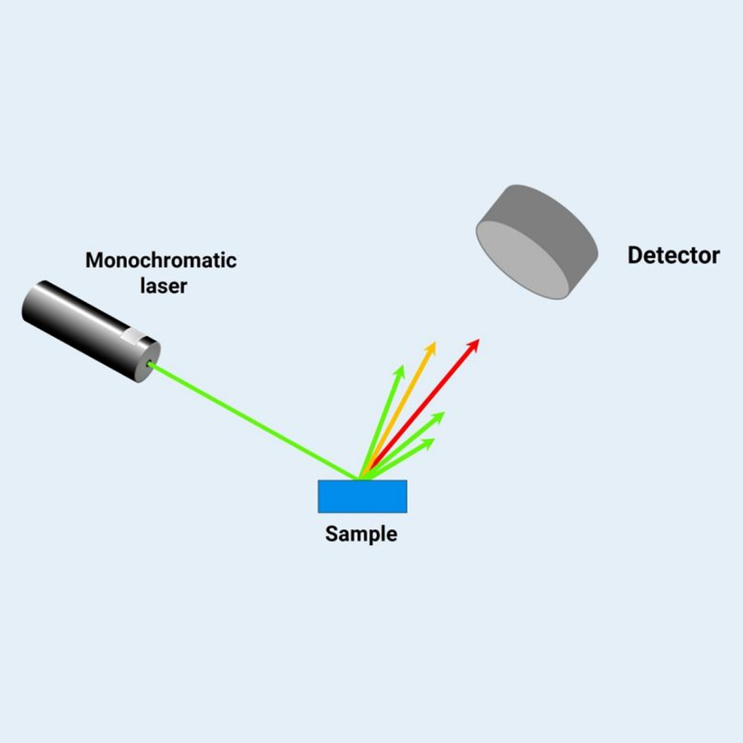
Raman spectroscopy measures inelastic light scattering. A focused laser illuminates the particle, and a small fraction of the scattered photons returns at shifted frequencies that encode the vibrational modes of the material. The chemical fingerprint this produces is physically distinct from an IR spectrum and sensitive to different molecular and inorganic bond symmetries, making Raman a complementary method of investigation.
In routine microplastics workflows, the standard implementation is still point-based: particles are localized optically and then measured at one or multiple positions. However, Raman imaging is possible, and with laser line imaging it becomes substantially more practical.
Raman microscopy is strongest when the required particle size range extends below what IR techniques can reliably characterize, or when inorganic fillers and mineral components are central to the analytical question. For sub-micrometer particles, nanoplastics, and chemically complex particles, Raman micro-spectroscopy and especially Raman laser line imaging provide capabilities that IR-based methods cannot replace, but for routine high-throughput full-filter analysis above the IR size range, FT-IR imaging or IR laser imaging will be more efficient.
Raman Micro-Spectroscopy
In point-based Raman micro-spectroscopy, particles are first localized optically. The instrument then acquires a Raman spectrum from selected particles or from selected positions on a particle. This workflow is widely used because it is flexible, chemically specific, and capable of analyzing particles below the reliable size range of IR-based techniques.
The defining capability of Raman microscopy is spatial resolution.
Because Raman uses visible or near-infrared laser excitation, the laser can be focused to a much smaller spot than mid-infrared radiation. This allows confident particle detection and characterization well below 1 µm, a region otherwise analytically invisible to IR-based workflows but one that is increasingly relevant to health research, because such particles can interact with biological barriers differently from larger microplastics.
Raman also excels at identifying inorganic components both within polymer particles and alongside them. Many real-world plastic particles contain inorganic fillers and additives, including calcium carbonate in polyethylene, talc in polypropylene, titanium dioxide as a whitening agent, carbon black, and glass fibre reinforcement.
These materials affect the spectral signature of the particle and can complicate polymer identification by other techniques. Raman’s sensitivity to inorganic bond symmetries allows it to characterise both the polymer matrix and its fillers. For discrete inorganic particles present alongside polymers in the sample, such as silica, glass, or calcium carbonate, the same applies. The same sensitivity to inorganic components creates a practical complication for filled polymers.
If a single Raman spectrum is collected per particle and the laser spot lands on a filler-rich region, the filler signal can dominate while the underlying polymer matrix is underrepresented, unidentified, or misclassified. A robust identification of filled or heterogeneous particles may therefore require several measurement points across the particle surface, with the resulting spectra averaged to obtain a representative signal. This brings the core constraint of point-based Raman micro-spectroscopy into focus.
Raman point analysis inherits the same limitations discussed for other micro-spectroscopic workflows. The particle population is defined before chemical analysis, making the workflow vulnerable to optical detection bias. Traceability is also limited because the analytical record consists of selected measurement points rather than a complete chemical dataset of the particle population or filter area.
Thus, scalability is a major issue. A typical Raman measurement may take a few seconds per point. A filter carrying several thousand particles can therefore require hours of acquisition time even at one point per particle. If particle averaging is required for filled or heterogeneous particles, the number of measurement points increases, and the measurement time multiplies accordingly. For complex samples where reliable identification of filled polymers matters, the time requirement can become substantial.
Fluorescence is the second major limitation. Many environmental samples contain materials that fluoresce strongly under laser excitation. Because the Raman signal is inherently weak, the fluorescence background can overwhelm the spectrum entirely. Careful substrate selection, laser wavelength optimization, and sample preparation can reduce this risk, but Raman workflows generally require more method development attention than IR-based imaging workflows.
Raman Imaging
Raman imaging extends Raman microscopy beyond single-point particle identification. Instead of acquiring only one spectrum from one position on a particle, the particle or a selected sample area is scanned systematically. The result is a spatially resolved Raman dataset that can show how chemical components are distributed across the particle or region of interest.
This is particularly valuable for heterogeneous particles. Real-world microplastics are often weathered, contaminated, pigmented, filled, or multilayered. A single Raman spectrum may represent only the exact point where the laser was focused. If that point is dominated by a filler, pigment, surface residue, or inorganic inclusion, the polymer matrix may be underrepresented or missed entirely. Raman imaging reduces this risk by measuring multiple positions across the particle.
The resulting dataset can be used in two ways. First, it can generate chemical maps that show the spatial distribution of polymer, filler, additive, residue, or inorganic material within or around the particle. Second, spectra from all relevant pixels or measurement positions can be averaged to obtain a more representative particle spectrum for classification. This makes Raman imaging especially useful for complex particles where one-point measurement is not sufficient.
Classical Raman mapping usually acquires spectra point by point. This makes it powerful for individual particles, inclusions, multilayer structures, and selected regions of interest, but slow when extended to large filter areas or complete particle populations. Acquisition time increases with the number of measured positions.
Laser line imaging, however, changes this practical balance. Instead of focusing the laser into a single spot and measuring one point at a time, the laser is shaped into a line, collecting 400 measurement points along that line in a single scan. This allows Raman imaging datasets to be acquired more efficiently than with conventional point-by-point mapping, while preserving the high spatial resolution that makes Raman valuable.
It does not remove all Raman-specific challenges (e.g. fluorescence, substrate choice, sample preparation, and acquisition settings still matter) but it makes Raman substantially more powerful than single-point spectroscopy for complex particles.
Technologies at a glance: FTIR vs ILIM vs Raman
| FT-IR Imaging | IR Laser Imaging (ILIM) | Raman Micro-Spectroscopy | |
| Particle size range | micrometer | micrometer | nanometer |
| Throughput | High — 25 mm filter in 3.5 hours | Ultra high — 25 mm filter in ~30 min, 20+ filters/day | Low — ~2 sec per measurement point, scales with particle count and complexity |
| Robustness | Very high — ML model trained on degraded, contaminated, and filled real-world polymers; performs well across complex environmental samples | High — same ML pipeline as FT-IR imaging | Variable — fluorescence from sample matrix or substrate can overwhelm the Raman signal; requires method development and careful substrate selection |
| Spectral coverage | Full MIR (4000–600 cm⁻¹ with silicon filter) | Fingerprint region only (1800–1250 cm⁻¹) | Full range (200–3500 cm⁻¹ Raman shift) |
| Polymer identification | Excellent | Excellent | Excellent |
| Inorganics (Fillers, Additives, Silica, ...) | Good - Discrete inorganic particles only with silicon filter | Good - Not reliable for discrete inorganic particles | Best - Sensitive to inorganic bond symmetries IR cannot detect |
| Automation | High | End-to-End | Partial — particle averaging and complex samples require more setup |
#7 Microplastics Data Evaluation
A micro-spectroscopic measurement produces a lot of raw data, and the step from raw spectra to a particle list with identity, size, shape, and count cannot be handled manually. Whether that data comes from millions of IR spectra across a complete filter or from point and area measurements collected particle by particle in Raman, does not matter.
Why manual evaluation and library matching both fail
With such immense data sets ranging from thousands to millions of spectra, manual evaluation is very slow - if not impossible. On top, environmental microplastics are not pristine. UV degradation, chemical weathering, adsorbed organic matter, and inorganic filler contributions all distort spectra away from the reference in ways that simple reference matching cannot reliably handle. Identification accuracy degrades precisely when the samples are most analytically demanding, and the degradation is not always visible to the user.
How AI-based classification works and where it depends on training data
An AI trained on large, diverse datasets of real-world microplastic spectra does not compare spectra to fixed templates. It learns the underlying spectral patterns associated with each polymer class, patterns that remain recognisable even under degradation and with contaminations and filler contributions present. This applies to both IR imaging and Raman classification pipelines.
The quality of the training data determines whether the model works on your samples. A model trained on clean laboratory reference material will perform well in the lab and poorly in the field. A model trained on verified real-world spectra across diverse polymer types, degradation states, and sample matrices will maintain classification accuracy where it needs to.
Automated classification is only useful if each result carries a reliable measure of how well the measured spectrum actually matches the assigned polymer class. A confidence score does this by taking the spectral feature vector extracted from the particle — the set of numerical values the neural network derives from the spectrum — and correlating it against the feature vector of a verified reference spectrum for that polymer class in a high-confidence library. The closer the correlation, the higher the score. Particles that fall below a user-defined threshold are excluded from the classification results.
This threshold is a methodological decision, as a high threshold accepts only particles with a strong spectral match, reducing false positives at the cost of potentially excluding degraded or contaminated particles that the model has correctly identified but with lower certainty. A lower threshold includes more particles but also increases the risk of misidentification. The right setting depends on the scientific question, the sample type, and whether the regulatory context places greater weight on sensitivity or on specificity.
How Bruker solves this
Bruker's MP-ID software handles this classification pipeline within OPUS, the instrument's operating software, without requiring a separate processing step or data export. After measurement, MP-ID divides the hyperspectral image into overlapping tiles, extracts spectral feature vectors pixel by pixel using a neural network, and assembles connected pixels of common identity into individual particles. A particle average spectrum is calculated for each, and the resulting feature vector is correlated against a dedicated high-confidence reference library to produce the HIT score. The default threshold is 800. Particles below that value are suppressed from the classification results; the threshold is adjustable based on the analytical requirements of the application. The open architecture of the software permits users to add new reference spectra to the library, if required by their specific analytical needs.
The model currently classifies all current / relevant polymers including: ABS, EVAc, PA, PC, PE, PEEK, PET, PLA, PMMA, POM, PP, PS, PU, PVC, SAN, Cellulose, and CaCO3. It is trained on verified reference data measured on LUMOS II and is designed to maintain classification accuracy across degraded, contaminated, and filled real-world particles. MP-ID is available as a subscription, which means the model is updated continuously as new training data and polymer classes are added, with the user having continuous access to the latest developments and improvements. The automated MP-ID classification algorithm is available for FT-IR and ILIM imaging datasets.
#8 Regulatory Landscape
Regulatory frameworks now increasingly reference spectroscopic particle analysis. Several international standards and regulatory frameworks now specify or reference spectroscopic methods directly. Laboratories need to know which frameworks apply, what they require, and whether they are binding or still in development.
EU Drinking Water Directive 2020/2184
EU Directive 2020/2184 on the quality of drinking water requires member states to monitor microplastics in drinking water supplies. It does not itself specify analytical methods but mandates the European Commission to establish a watch list of substances requiring monitoring and to define the methods to be used. The analytical requirements are set out in the implementing act below.
EU Commission Delegated Decision 2024/1441
This is the implementing act under Directive (EU) 2020/2184 (the Drinking Water Directive) that defines a harmonised methodology for measuring microplastics in water intended for human consumption.
It specifies particle‑based characterisation using vibrational micro‑spectroscopy (including μFTIR, μRaman, and QCL‑IR microscopy), sets minimum requirements for particle size classification, defines polymer identification criteria, and establishes standardised reporting requirements.
For laboratories conducting microplastics analysis in drinking water under EU legislation, this Decision is the binding regulatory reference that defines what constitutes an acceptable analytical approach and compliant reporting.
ISO 24187:2023
ISO 24187:2023 defines general principles and minimum analytical requirements for microplastic analysis across environmental matrices, including water, sediment, and biota.
It recognises vibrational micro‑spectroscopy, including IR (μFTIR) and Raman microscopy, as appropriate techniques for the chemical characterisation of microplastic particles. The standard addresses key aspects of method development, validation principles, quality assurance, and reporting, without prescribing specific monitoring programmes or regulatory thresholds.
ISO 24187 serves as a foundational reference for laboratories developing robust and transparent microplastics analysis methods across environmental applications.
ISO 4484-2:2023
ISO 4484-2 addresses microplastic analysis specifically in textiles and textile products by FT-IR spectroscopy. It provides application-specific methodology for a regulated product category and is the relevant reference standard for laboratories working in the textiles sector.
ISO 16094-2:2025
ISO 16094-2:2025 specifies vibrational spectroscopy methods for microplastics analysis in drinking water and waters with low suspended-solids content. It covers particle sizing, counting, size classification and chemical identification using microscopy coupled with vibrational spectroscopy. It complements ISO 24187:2023 with more specific requirements for these water matrices.
ASTM WK87463
ASTM WK87463 is a work item under development by ASTM International's D19 water committee. It will provide a test method for the spectroscopic identification and quantification of microplastic particles in water using IR spectroscopy, covering FTIR, laser direct IR imaging, and equivalent techniques capable of measuring IR spectra from particles in the 20 µm to 5 mm size range. It is not yet published. When finalised it will be the primary ASTM reference method for IR-based microplastic analysis in water, relevant particularly for North American regulatory and compliance contexts.
#9 Supporting and Confirmatory Spectroscopic Techniques
Some spectroscopic methods are better suited to confirmation and screening than to population-level particle metrics. In addition to imaging‑based methods, targeted spectroscopic techniques are widely used to support, verify, or screen particles selected from a sample. These approaches provide chemical identification for individual particles but do not aim to characterise entire particle populations.
Targeted particle spectroscopy relies on manual selection of visually identifiable particles followed by single‑particle chemical analysis. Two techniques are commonly used in this role: ATR‑FT‑IR particle spectroscopy using benchtop instruments, and handheld Raman spectroscopy.
In ATR‑FT‑IR particle spectroscopy, individual particles are isolated, typically under a stereomicroscope, and placed in direct contact with an attenuated total reflection crystal on a benchtop FT‑IR spectrometer. Infrared radiation interacts with the particle via an evanescent field at the crystal surface, producing a spectrum characteristic of the material. The method is non‑destructive and provides robust polymer identification for the particles that are measured.
Handheld Raman spectroscopy follows a similar analytical logic but uses portable, battery‑powered instruments. A focused laser is directed onto a selected particle, and the inelastically scattered light is analysed to generate a Raman spectrum. Measurements can be performed directly on particles on filters, in containers, or in the field, with minimal sample preparation.
In both cases, the analytical output is limited to chemical identity for selected particles only. Because particles are chosen manually, these techniques do not provide systematic information on particle abundance, size distribution, or morphology across the sample. Measurement time scales directly with the number of particles analysed, and operator selection introduces an unavoidable bias toward visually conspicuous particles.
The principal strength of these approaches lies in practicality and accessibility. Benchtop ATR‑FT‑IR instruments are widely available, relatively low in cost, and straightforward to operate, while handheld Raman instruments enable rapid, on‑site screening without laboratory infrastructure. Both techniques can reliably identify common polymers in larger particles and are well suited to confirmatory analysis, method development, training, and quality control. ATR‑FT‑IR is particularly robust for thick, irregular, dark, or opaque particles, while handheld Raman offers unmatched portability and speed for rapid screening.
Their limitations are equally well defined. Small particles, typically below approximately 20 to 30 micrometres, are difficult to manipulate for ATR‑FT‑IR and may not establish sufficient contact with the ATR crystal. Handheld Raman instruments are constrained by optical resolution and are generally limited to particles larger than roughly 50 to 100 micrometres. Fluorescence frequently interferes with Raman measurements, particularly for environmental samples containing pigments, additives, or organic residues. In both cases, quantitative analysis and statistically representative results are not achievable.
Because targeted particle spectroscopy does not deliver particle counts, size‑resolved composition data, or full‑sample coverage, it does not align with regulatory and monitoring frameworks that require particle‑based metrics derived from population‑level analysis. These techniques therefore function as supporting and screening tools, rather than as standalone solutions for routine monitoring or compliance testing.
In microplastics workflows, ATR‑FT‑IR particle spectroscopy and handheld Raman are most effective when used in combination with particle‑resolved imaging techniques. They support verification of unusual particles, rapid screening of samples, and confirmatory identification, while imaging‑based methods provide the statistically representative data required for environmental monitoring, exposure assessment, and regulatory reporting.
- Tap water (87%, more recent)
Bian, Z. et al. (2024). Global prevalence of microplastics in tap water systems: Abundance, characteristics, drivers and knowledge gaps. Science of the Total Environment. https://doi.org/10.1016/j.scitotenv.2024.172086 - Bottled water (93%)
Mason, S.A., Welch, V.G., Neratko, J. (2018). Synthetic Polymer Contamination in Bottled Water. Frontiers in Chemistry, 6, 407. https://doi.org/10.3389/fchem.2018.00407 - Human lung tissue
Jenner, L.C. et al. (2022). Detection of microplastics in human lung tissue using μFTIR spectroscopy. Science of the Total Environment, 831, 154907. https://doi.org/10.1016/j.scitotenv.2022.154907 - Human blood
Leslie, H.A. et al. (2022). Discovery and quantification of plastic particle pollution in human blood. Environment International, 163, 107199. https://doi.org/10.1016/j.envint.2022.107199 - Human placenta
Ragusa, A. et al. (2021). Plasticenta: First evidence of microplastics in human placenta. Environment International, 146, 106274. https://doi.org/10.1016/j.envint.2020.106274 - PyroGC
Primpke, S. et al. (2020). Critical Assessment of Analytical Methods for the Harmonized and Cost-Efficient Analysis of Microplastics. Applied Spectroscopy, 74(9), 1012–1047. https://doi.org/10.1177/0003702820921465 - TRWP
Fraunhofer UMSICHT. (2024). Microplastics: Tire and road abrasion — Tire and road abrasion in the focus of a new publication. Fraunhofer Institute for Environmental, Safety and Energy Technology UMSICHT. https://www.umsicht.fraunhofer.de/en/press-media/press-releases/2024/reifen-und-fahrbahnabrieb.html - Nanoplastics & Blood-Brain-Barrier
Kopatz, V. et al. (2023). Micro- and Nanoplastics Breach the Blood–Brain Barrier (BBB): Biomolecular Corona’s Role Revealed. Nanomaterials, 13(8), 1404. https://doi.org/10.3390/nano13081404