Determination of Metal Coating Layer Thicknesses in Cultural Heritage Using a Reference-Based Approach
Whether it is gildings, silverings or tinnings: in Heritage Science we often come across metal coatings on a variety of different materials ranging from polychrome wooden panels to book illuminations or metal objects. Understanding the properties of these coatings aids the understanding of historical technologies used to produce the objects or in provenance studies. One of the key properties of metal coatings is the coating thickness which, depending on the application technique and production date, can vary strongly.
The coating layer thickness can be easily determined with micro-XRF (X-Ray Fluorescence). One may wonder how this is possible using a non-invasive technique? Well, the coating thickness actually cannot be determined directly by XRF, but by the number of atoms! The coating thickness is just a function of the density at which the atoms are deposited on the object or sample.
The coating thicknesses discussed here can be penetrated by the primary X-ray beam – giving us the most crucial determinant when discussing XRF analysis: the information depth. The information depth can be defined as the depth from which 90 % of the generated element fluorescence radiation can escape the sample. It depends on the energy of the emission line in question as well as the average density of the material analyzed.
Practically, when looking at the gilded panel of Fig. 1, we are only able to see the gilded surface with our eye (VIS), while the X-rays reveal the Ca-rich priming (Ca-Kα) covered by an Fe- and Mn-rich bole (Fe-Kα and Mn-Kα), which is the base for the subsequently applied gold leaves using the poliment gilding technique.
As can be seen in the graph with calculated information depths of various XRF emission lines, the gilding must be thinner than 9 µm, as we can detect characteristic line of Ca and Fe below the gold layer.
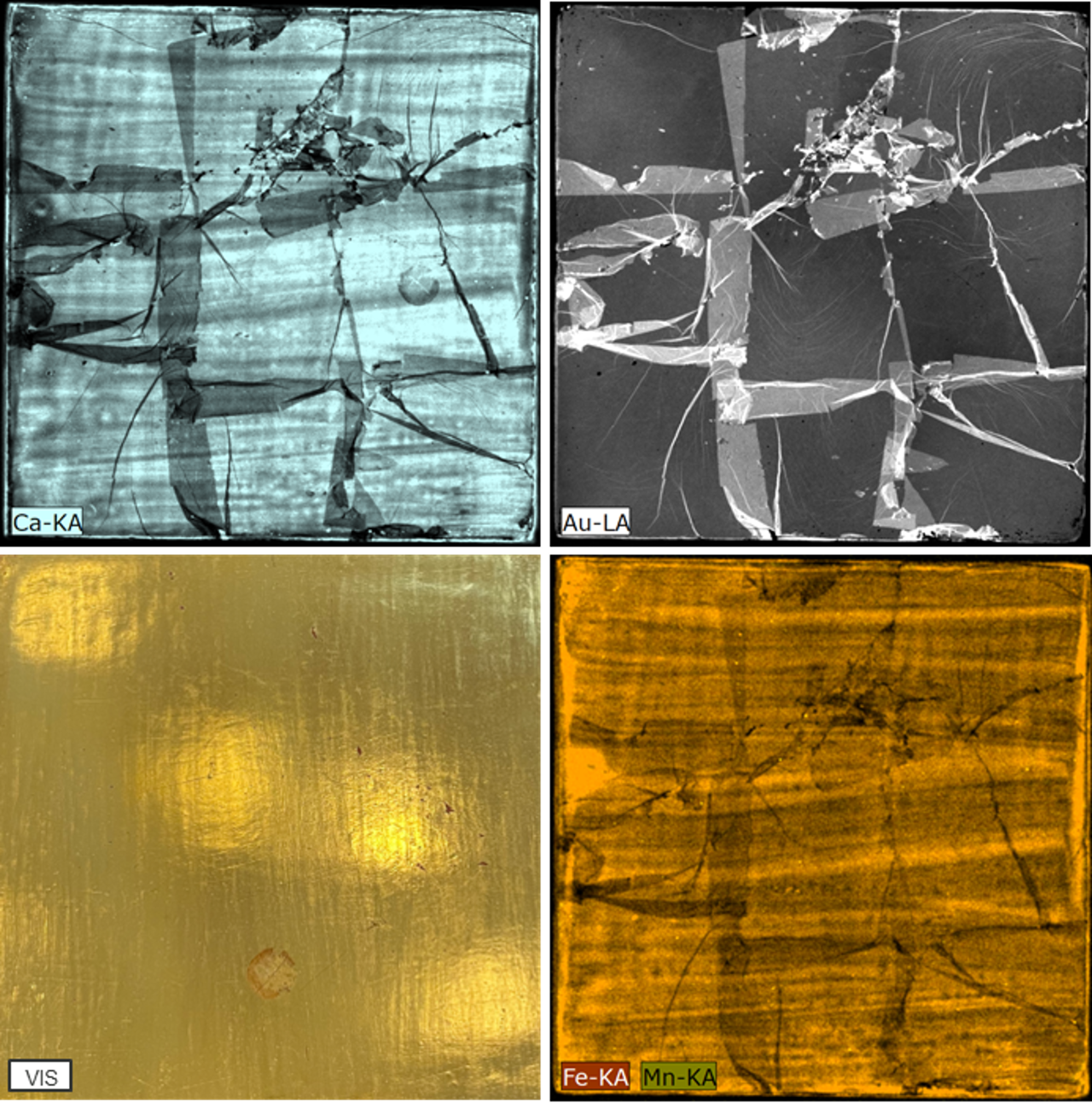
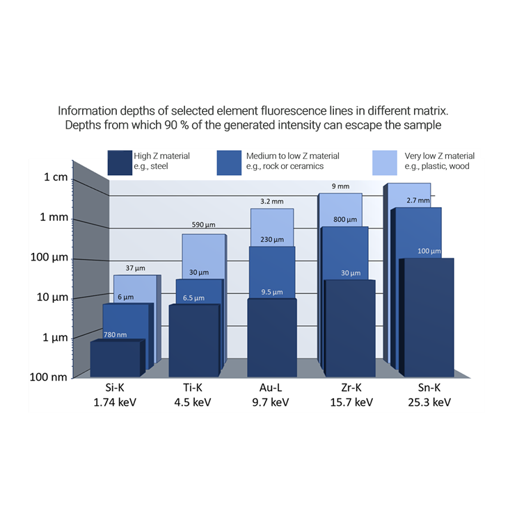
Fig. 1: Non-infinity of a poliment gilded panel and tabulated information depth for a selection of characteristic emission lines in different matrixes.
This becomes clearer when measuring reference materials made of gold foils of certified layer thicknesses (Fig. 2).These standards were analyzed on top of the prepared priming and bole to simulate a similar background as for our gilding. Measured coating thicknesses range from 0.053 µm up to c. 6 µm and show a clear saturation of the Au-L net intensity, the closer the layer thickness approaches the point of infinite thickness for the X-ray beam.
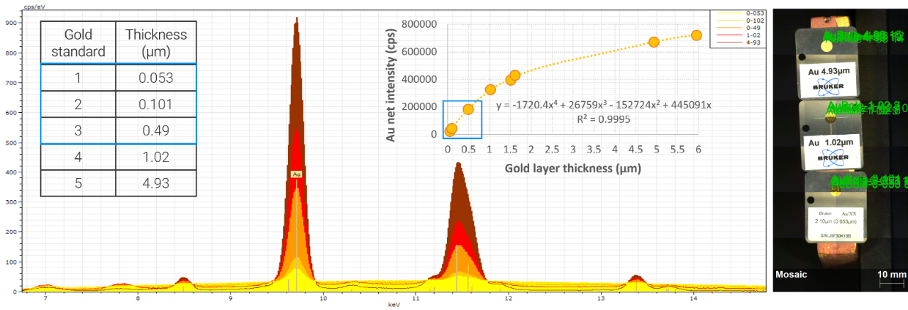
Fig. 2: Certified gold standards of varying thickness and their related intensities as measured with the M6 JETSTREAM. Net intensities are given in counts per second (cps) and are corrected for the detector dead time.
Regarding our poliment gilding, we are most interested in the sub-500 nm area of the curve (highlighted blue), as the common gold leave thickness ranges between 100 and 300 nm. Luckily, in this range the correlation of net intensity and layer thickness is linear, which makes extrapolation relatively easy (Fig. 3).
How can we apply these principles in practice? To calculate the gold coating thickness, we use a standard method from Analytical chemistry, the so-called “standard addition method”. This approach is based on using one or two reference materials of certified layer thickness, that are measured on top of the unknown analyte. This creates an “offset”, that allows to get the unknown coating thickness at the point where the trendline intersects the X-axes (Fig. 3).
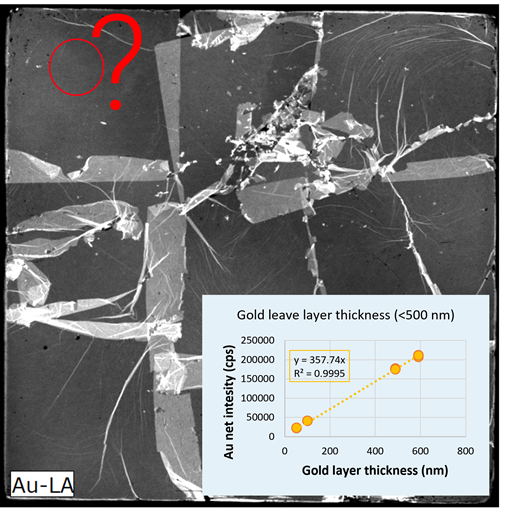
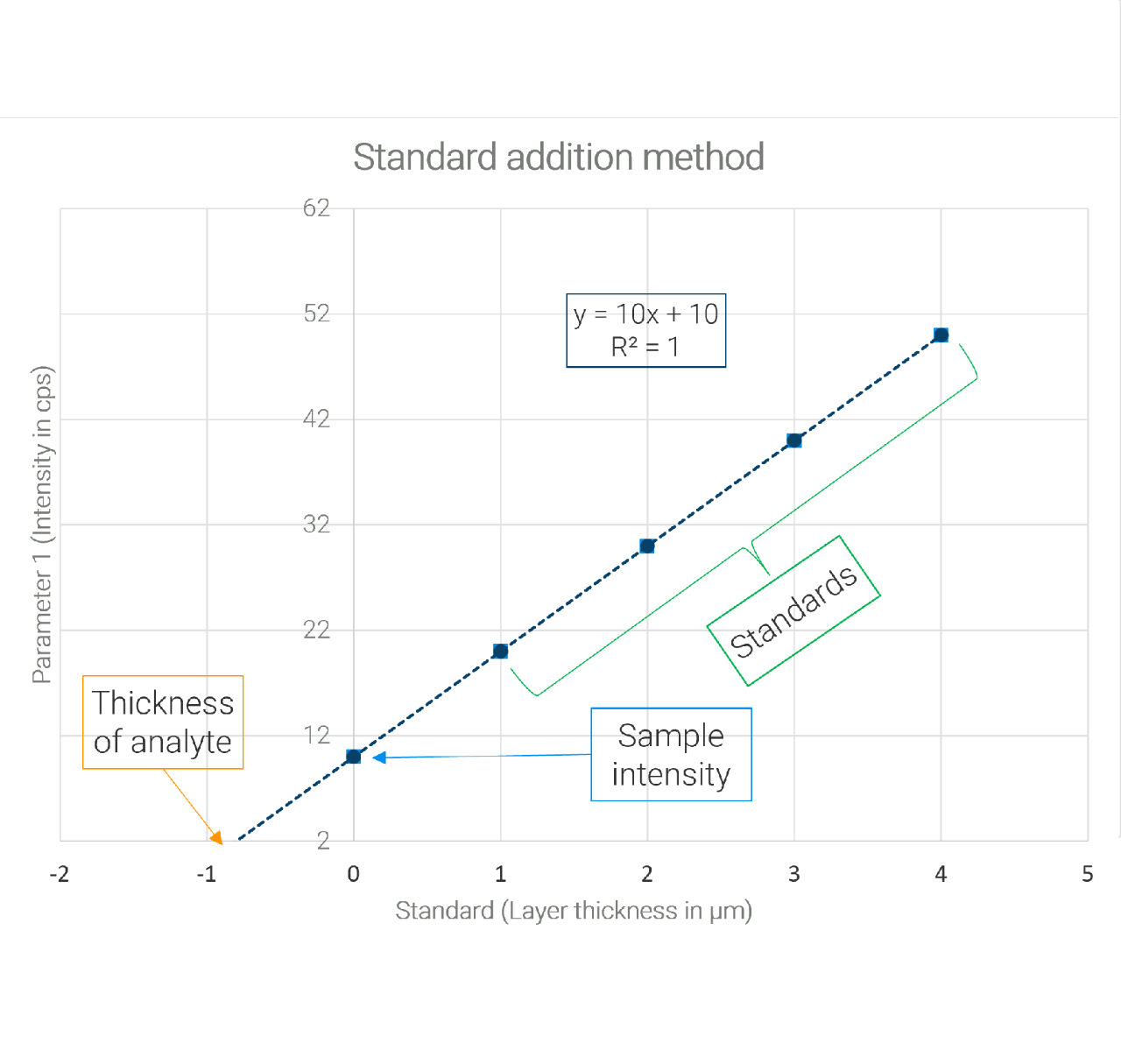
Fig. 3: Eased by a linear correlation, the gold leave thickness can be calculated using the Standard addition method.
On the gilded panel, we selected a suitable area based on the Au-Lα distribution measured via a micro-XRF scan with a 2 x 60 mm2 SDD M6 JETSTREAM (Fig. 3, red circle). On top of this area, two standards were placed one after the other and measured on four points. Afterwards, the exact same points were measured without any reference materials (Fig. 4).
Plotting the Au net intensity versus the layer thickness and using the resulting formula, we calculated a coating thickness of 133 nm. The deviation of ± 8 nm, that is based on variations of the net intensity, can be related to the uneven burnishing of the gold leaves after their application. Calculating further, this would be a variation of just 50 atoms!
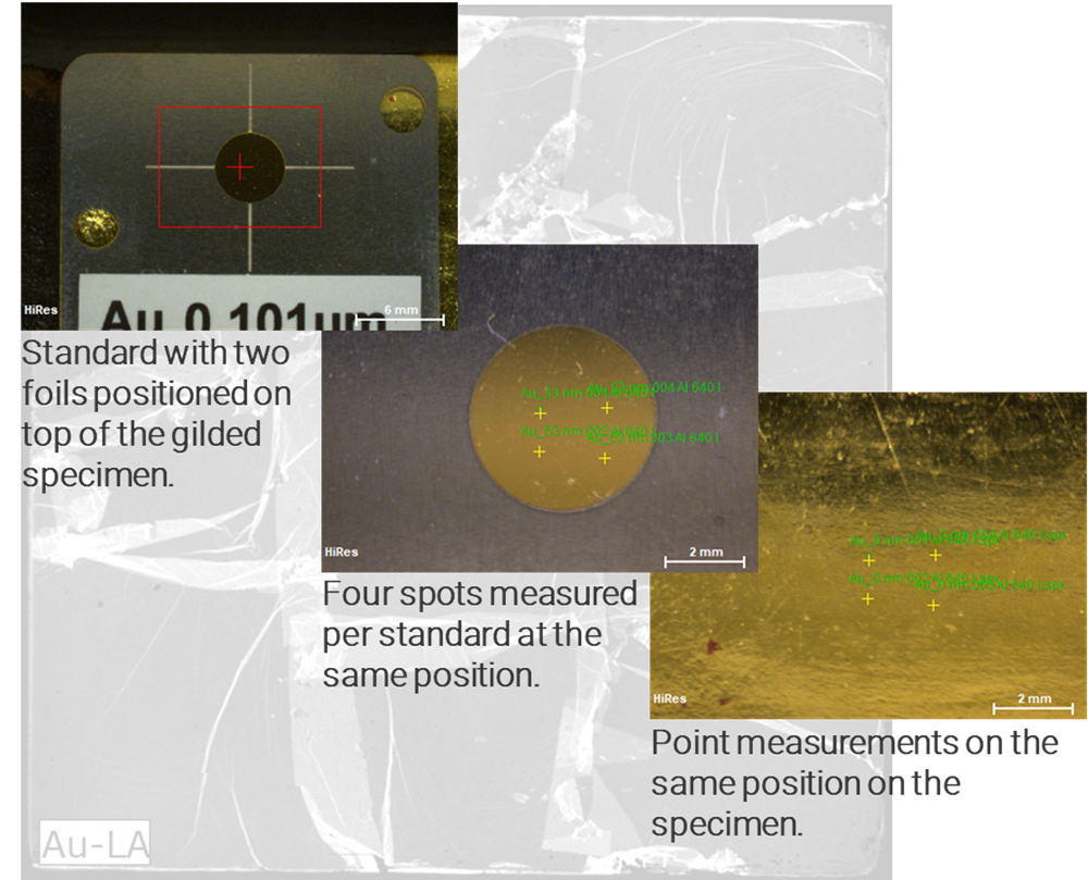
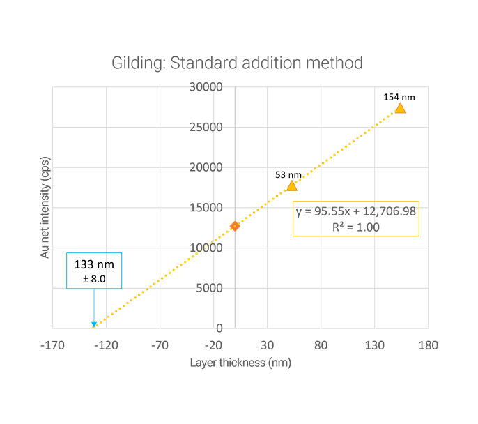
Fig. 4: The Standard addition method in practice: Gold foils of certified layer thickness were measured on top of the gilded panel at the exact same position. Using slope and offset of the linear correlation between Au net intensity (cps) and layer thickness (nm), a gold coating thickness of 133 nm ± 8 nm can be calculated.
The same principles can be applied to any type of metal coating, as shown below in the analysis of a tinning on top of a copper cauldron (Fig. 6). As long as there is a linear relation between the XRF intensity and the layer thickness, the standard addition method provides a quick and reliable workflow. In the case of the tinning, the point measured had a coating thickness of 3 µm.
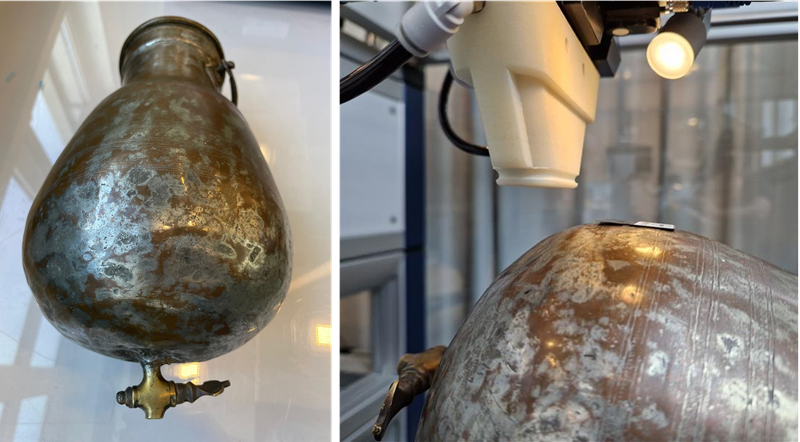
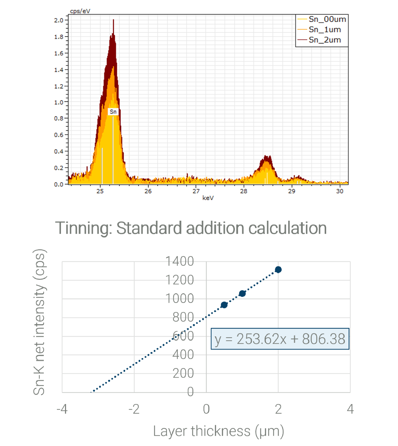
Fig. 5: The Standard addition method applied on a tinning of a copper cauldron.
To conclude, standard-based XRF analysis provides a quick and reliable workflow for the determination of coating thicknesses or mass deposits of a large variety of Cultural Heritage objects. The standard addition method can be performed using both certified reference materials or lab-developed samples. Creating references in the lab allows researchers to have full control of their results and calibrations.
For more information on this topic watch our on-demand webinar:
Remarks
Part of this Webnote was presented at the EXRS 2024 by Gerken et al.: https://exrs2024.demokritos.gr/